10 - Georg Umgiesser, "The impact of operating the mobile barriers in Venice (MOSE) under climate change" (2020)

 

Statistics of closures

 

In Fig. 3 the statistics of the total closures per year is shown. It can be seen how (depending on the type of closure, see Table 1) the number of closures rise from the actual situation with no SLR of 5–12 closures to 300–430 closures for a SLR of 50 cm, peaking at around 75 cm (550 closures) and leveling off at SLR higher than 140 cm to a little more

 

 

Table 1

Overview of simulations. For all types of simulations, 21 simulations have been carried out simulating a SLR from 0 to 2 m in 10 cm increment.

 

 

than 200 closures. The total number of closures using either the forecast or the exact water level (not available in the operational situation) are quite similar, but the number of closures that adds a 10 cm security increment is much higher, at least for smaller SLR. For SLR of more than 100 cm all curves coincide.

Not only the number of closures can be computed, but also the total time the lagoon stays closed during a closure. In normal situations, the closures should last an average of 4 h, but with higher SLR the period of closures become longer. Fig. 4 shows the statistics for the total time of

closure per year. The time of closure passes from the present situation of some hours (22–44) to about 1400−1800 hours with SLR of 50 cm, which is still compatible with the average of 4 h per closure. However, with higher SLR (over 140 cm) it reaches a plateau of about 8200 h. Since the year has 8760 h, the situation in which half of the time the lagoon is closed happens with a SLR between 70 and 80 cm. The periods with scenario FOR and OBS are nearly identical, and SEC is always higher. However, above 80 cm of SLR the curves coincide.

 

 

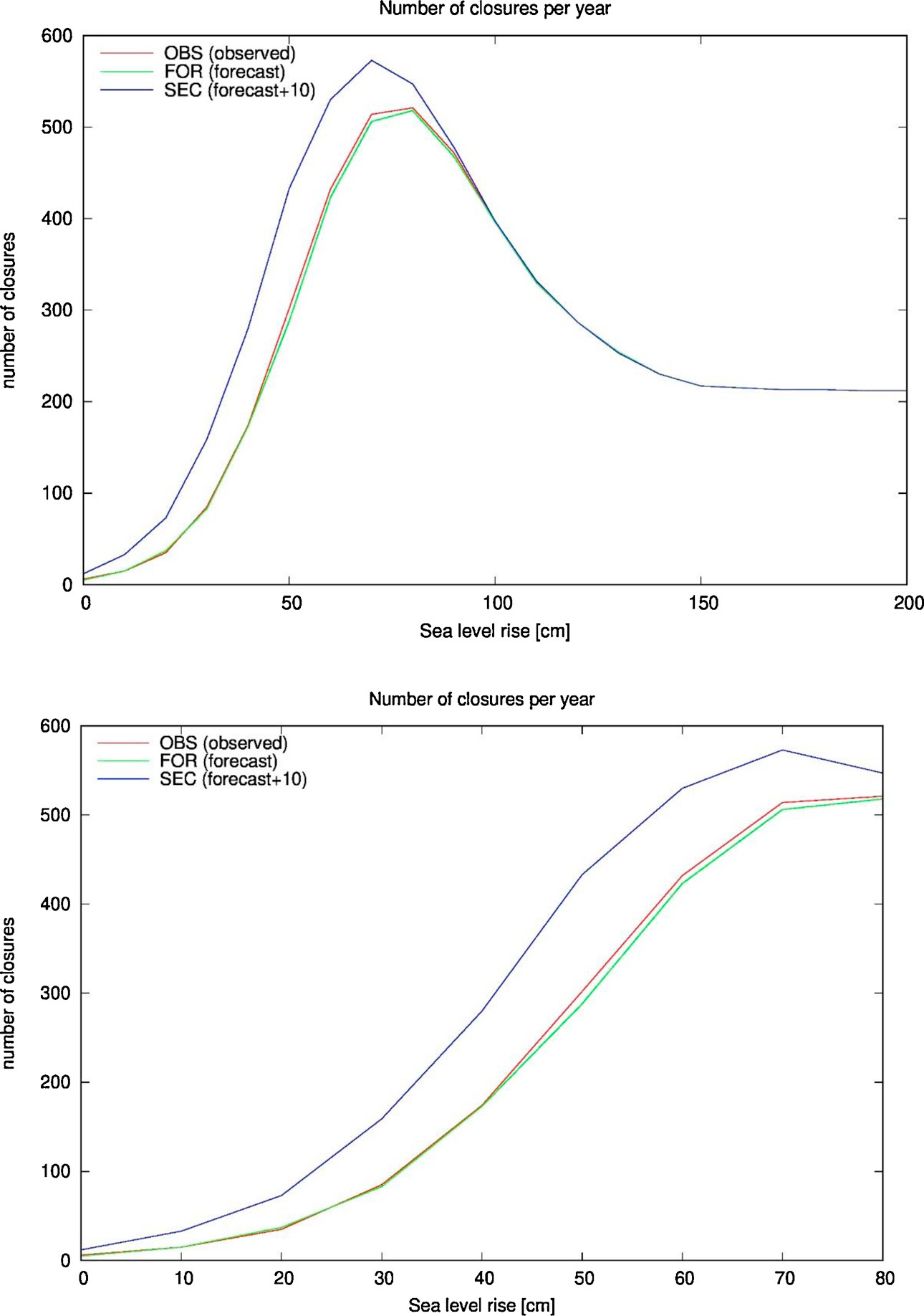
Fig. 3. Number of closures per year with different sea level rise and three different types of closure. Top shows SLR from 0 to 200 cm, bottom only the first 80 cm. The type of closure is described in Table 1.

 

 

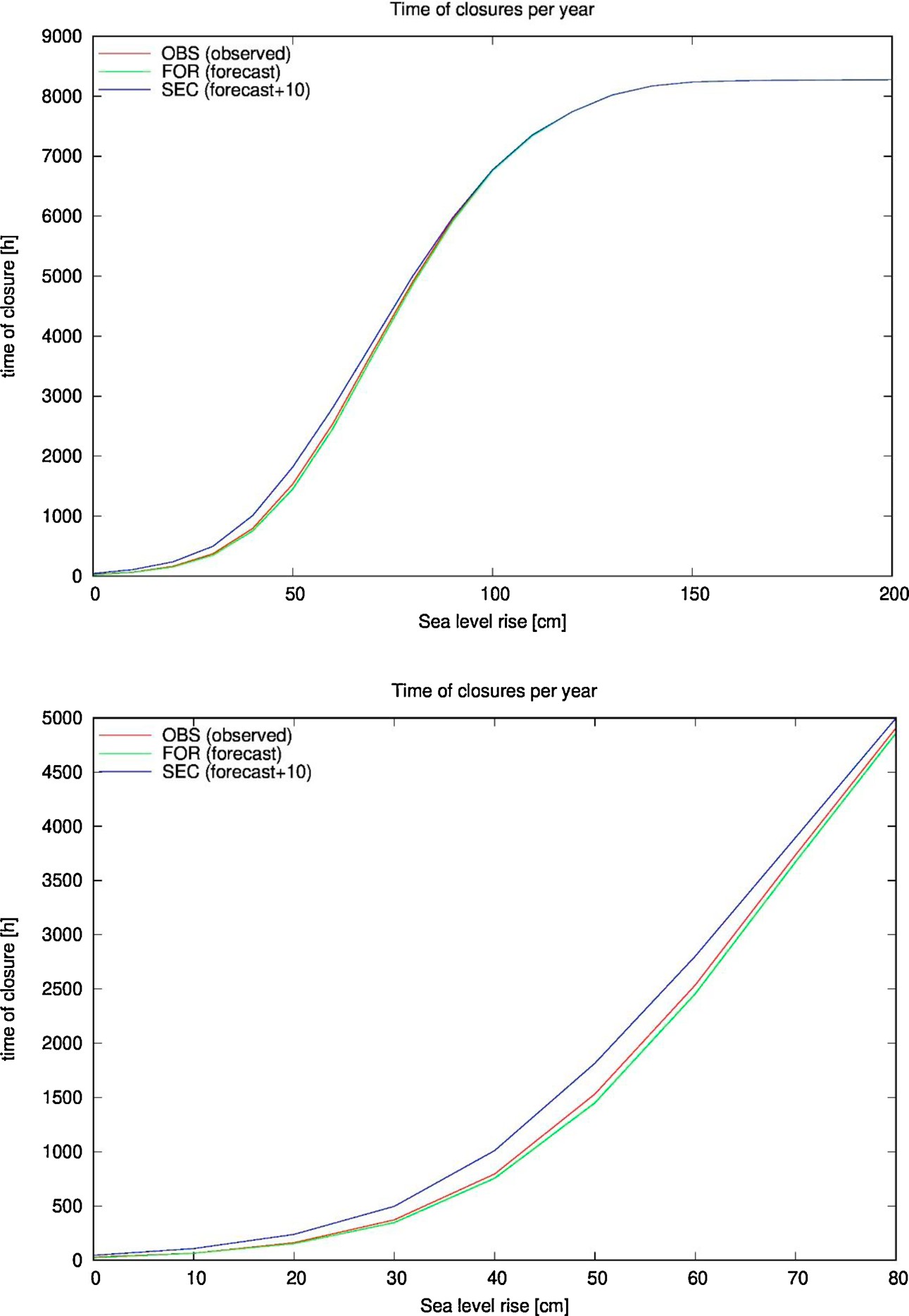
Fig. 4. Total time of closures per year with different sea level rise and three different types of closure. Top shows SLR from 0 to 200 cm, bottom only the first 80 cm. The type of closure is described in Table 1.

 

 

Over threshold

 

It can be also computed how many times and hours the water level in the lagoon rises over the threshold of the safeguarding level of 110 cm. This can happen because with the forecasted water level, errors in the forecast could lead to non-closures. It can also happen because in some cases, even with the lagoon closed, the water level rises due to the discharges of rivers and precipitation, and also due to leakage through the closed gates. Fig. 5 shows the results. In the present case, the mobile barriers can effectively protect the city, and only in a negligible number of hours the water level rises higher than 110 cm (6 h in the worst case). With a SLR of 30 cm these numbers rise to between 5−30 hours, and with 50 cm to 18−100 hours (35 h for the OBS scenario). However, above a certain SLR (here 100 cm) the curve starts to rise strongly and reaches at about 160 cm the value of 8600 h, nearly the whole time of the year. At this level of SLR (100 cm) the average sea level in the sea is 20 cm higher than the safeguarding level at which the MOSE has to be closed. This means that only at low tide the gates can still open, and the lagoon fills up continuously with water coming from the sea.

These numbers should be compared to the time over threshold when the mobile barriers are not active (REF curve in Fig. 5). The number of hours rises steeply already with smaller SLR values. With a SLR of 50 cm Venice would be flooded for more than 1000 h.

 

Fluxes through the inlets

 

Closing the mobile barriers certainly also has an effect on the water exchanges through the inlets. The exchange will then depend through the numbers of closures also on the SLR. With the simulations it is possible to compute the average water flux through the inlets. In the present case, and without closures (REF), the discharge is 4654 m³/s (daily average over simulation). When the mobile barriers are active, in the present case without SLR, the discharge reduces a little to between 4622−4637 m³/s, depending on the scenario.

Fig. 6 shows the dependence of the discharge on the SLR. Without any closures the discharge is rising continuously with rising SLR values. However, when considering closures of the mobile gates, with low le-vels of SLR the discharge rises to a level of about 4850 m³/s for about

 

 

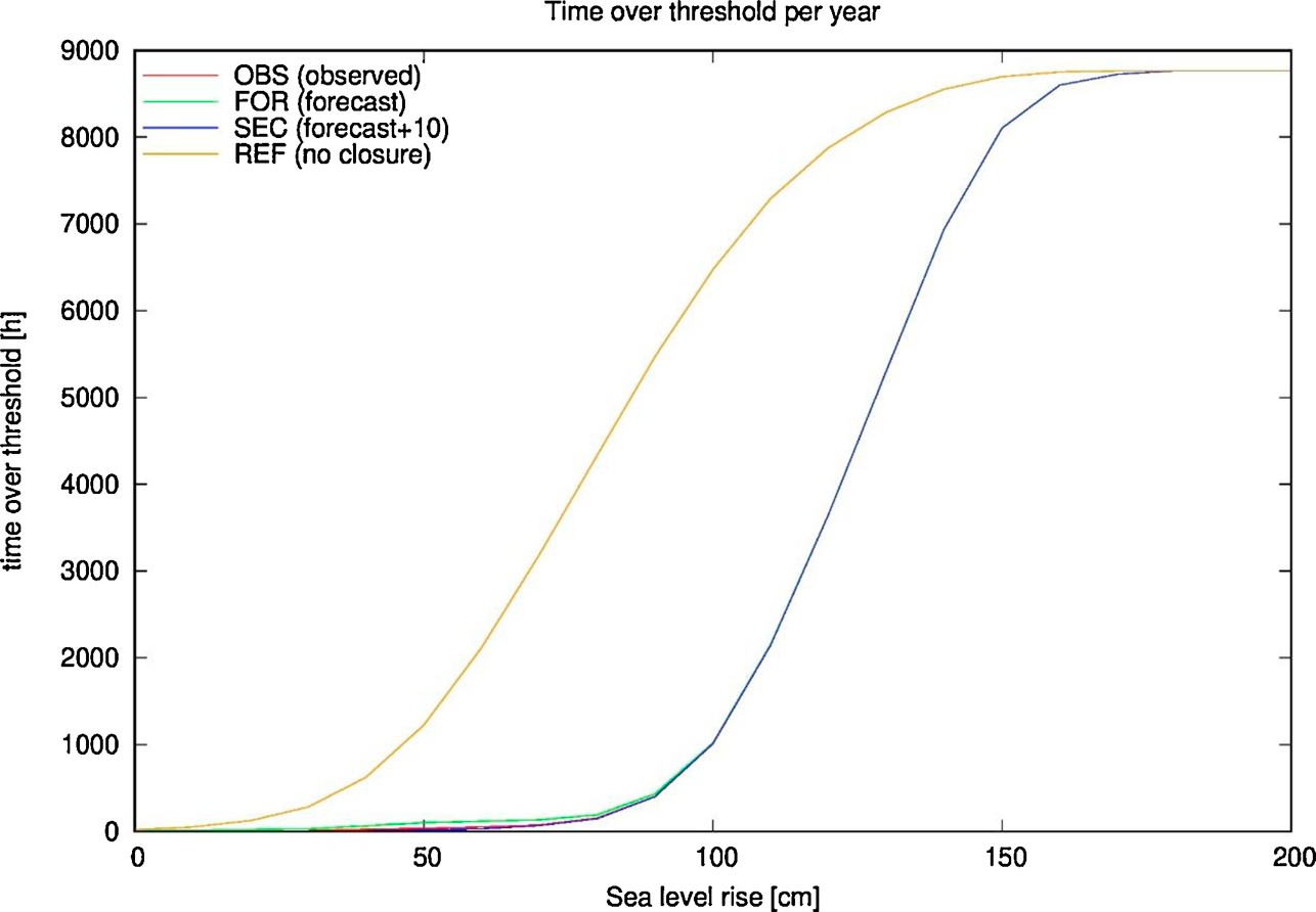
Fig. 5. Total time of flooding over threshold per year with different sea level rise and three different types of closure. The threshold here is 110 cm. The type of closure is described in Table 1.

 

 

20−30 cm of SLR, and after this level the discharges start to decrease strongly. At a SLR of over 150 cm the discharges stabilizes at a level of about 160 m³/s.

 

Partial closures

 

In the above simulations the mobile barriers have been used in an all or nothing mode: either they are open or they are closed all together. There is however also the possibility of a partial closure, where some inlets are closed and others are kept open. Here two cases have been studied: the case where only the Lido inlet (the northern one) will be closed (OLI) and the case where the other two inlets will be closed and only Lido will be open (NLI). The Lido inlet has been chosen for this experiment, because it is the closest inlet to the historic city, and therefore considered the most important one for high water.

Results can be seen in Fig. 7 as a scatter diagram. Only one situation is shown that will make the point for the other ones. Here a SLR of

50 cm and a security increment of 10 cm have been adopted. The figure shows that, without closures (REF) the water level inside the lagoon is slightly amplified with respect to the levels outside the lagoon. If a total closure is made, the safeguarding level of 110 cm can be defended in almost all instances. Only for an average of 18 h per year the level of 110 cm is exceeded, and only in one instance the water level reaches 120 cm. This is certainly a sign that in almost all events the MOSE is able to defend the city from high water.

If the lagoon is only partially closed (either only Lido or only the other two inlets), a significant reduction of the sea level cannot be achieved. As can be seen in the figure, the values inside the lagoon are more similar to the situation without any closure, and for a storm surge with values higher than 130 cm, basically all the water levels inside the lagoon are higher than the safeguarding level. The water level (average per year) will be higher than 110 cm for around 600 h (Lido only clo-sure) and 900 h (No Lido closure).

 

 

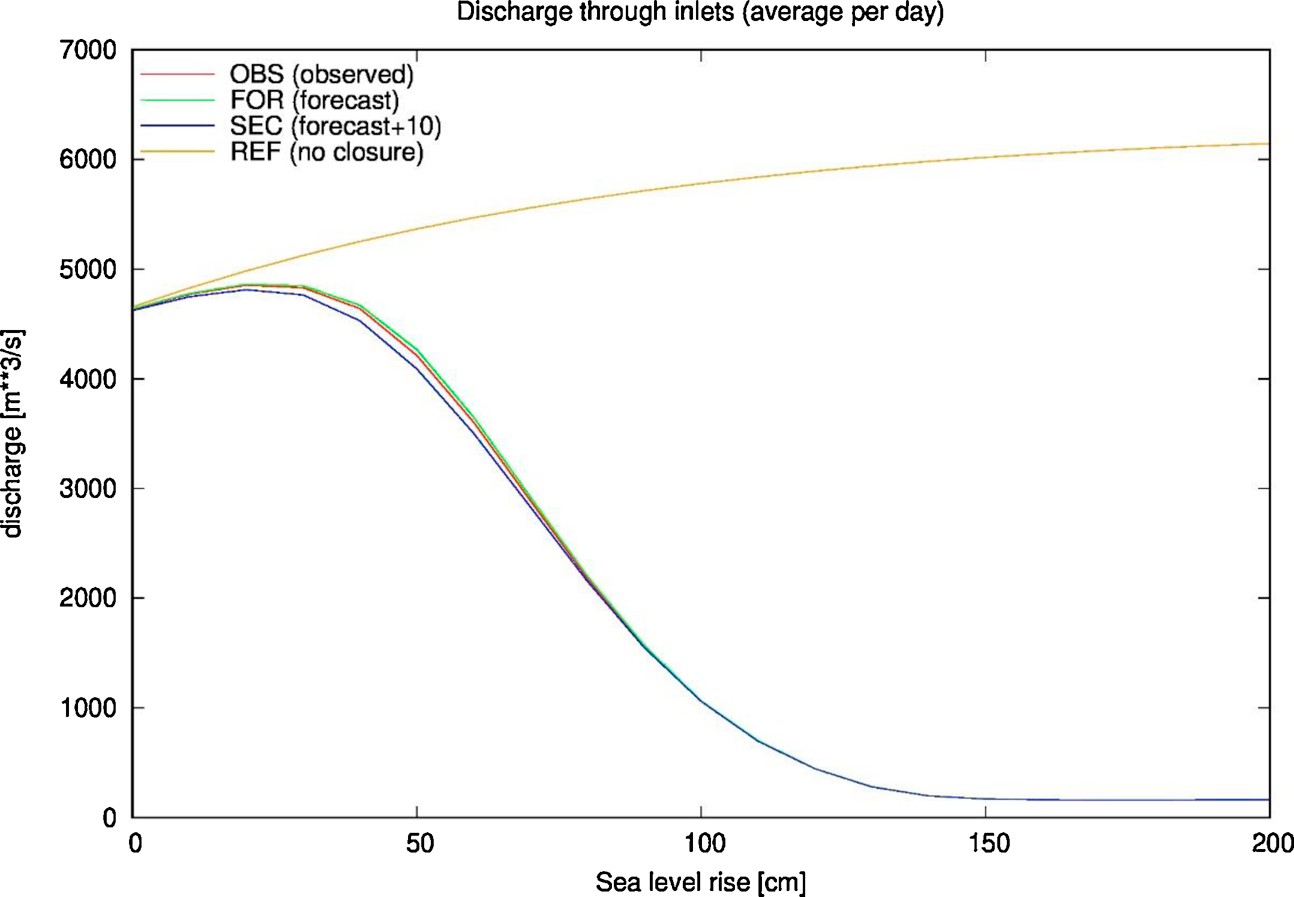
Fig. 6. Total discharge through inlets (daily average over simulation) with different sea level rise and three different types of closure. In addition, the discharge for the reference simulation (no closures) is also shown. The type of closure is described in Table 1.

 

 

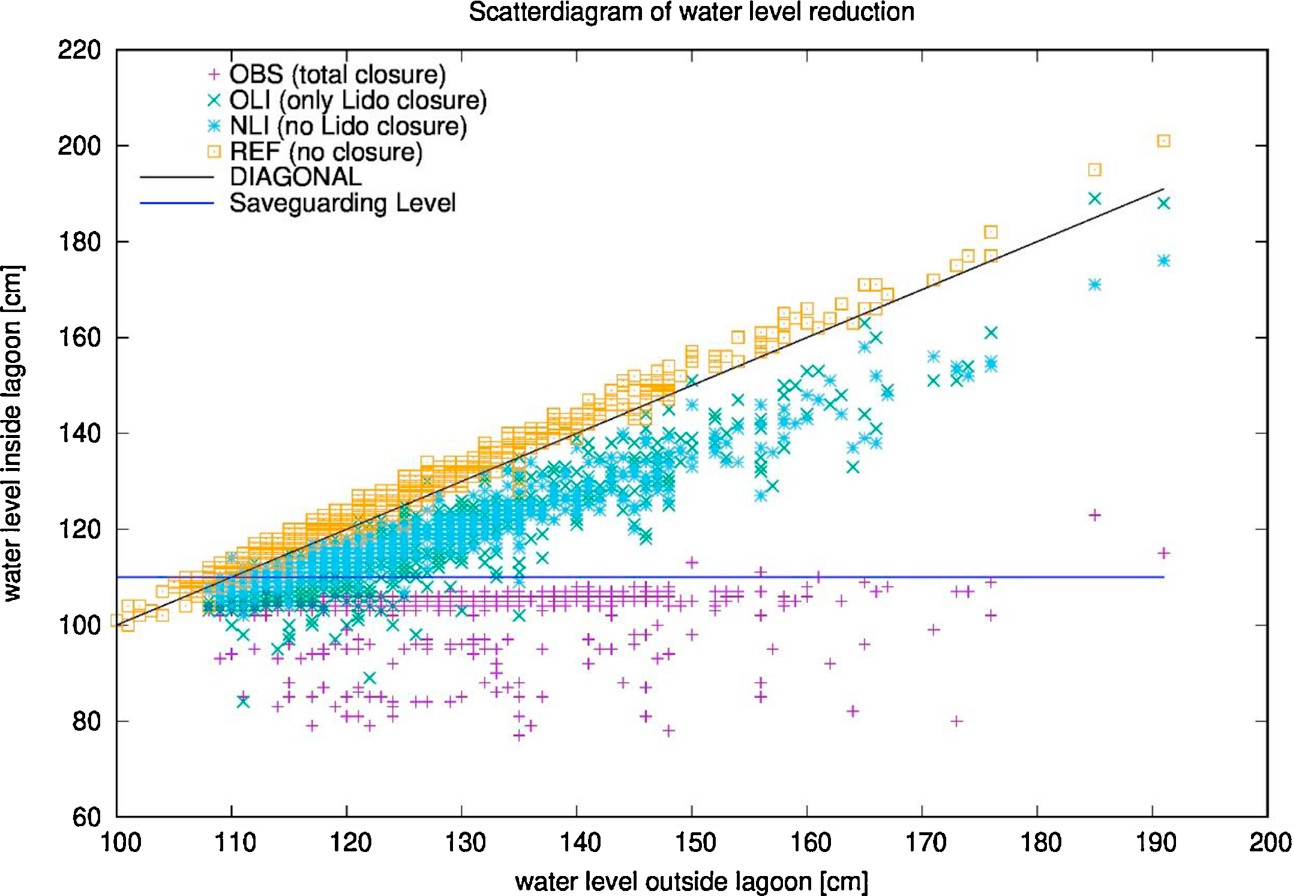
Fig. 7. Peak water levels outside and inside the lagoon for a SLR of 50 cm and different type of closures. The type of closure is described in Table 1. It can be clearly seen that a partial closure of the lagoon is not able to keep the water level below the safeguarding level.